```{r}
#| label: setup
#| include: false

data("Oats", package = "nlme")
(Oats <- as.data.frame(Oats))

# Pre-generate QR code image for title slide
png("qr-title.png", width = 300, height = 300)
qrcode::qr_code("https://github.com/Gelsleichter/quarto_ws/") |> plot()
dev.off()
```


<!----------------------------------------------------------------------
  BLOCO 0 — TITLE & INTRODUCTION
----------------------------------------------------------------------->

## About Me

::::: columns
::: {.column width="90%"}
**Yuri Gelsleichter**

- Postdoc Soil department — MATE, Gödöllő
- Background: Soil Science, Digital Soil Mapping, Pedometrics,
  Spectroscopy
- Daily tools: R, Quarto, Linux, GDAL, QGIS, JavaScript, Positron (VS
  Code-like)
- 📧 Gelsleichter.Yuri.Andrei\@uni-mate.hu
- 🔗 [github.com/Gelsleichter](https://github.com/Gelsleichter)
- 🔗 [research.uni-mate.hu/hu/w/dr.-gelsleichter-yuri](https://research.uni-mate.hu/hu/w/dr.-gelsleichter-yuri)
:::

::: {.column width="50%"}
:::
:::::

<!----------------------------------------------------------------------
  BLOCO 1 — THE PROBLEM
# Part 1: The Problem {background-color="#2C3E50"}
----------------------------------------------------------------------->

## Who Has Done This? 🙋

:::::: columns
::: {.column width="50%"}
1.  Run analysis in R / Python / Excel / SPSS
2.  Copy table → paste into Word
3.  Copy figure → paste into Word
4.  Adjust formatting, captions, numbering...
5.  Co-author says: **"Let's transform the data"**
6.  **Start over from step 1** 😩
:::

:::: {.column width="50%"}
::: fragment
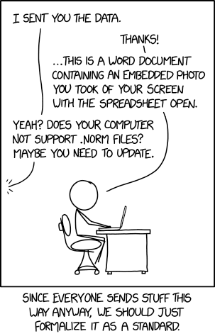![](https://imgs.xkcd.com/comics/norm_normal_file_format.png){width="60%"
fig-alt="xkcd comic about file formats"}
:::
::::
::::::

## The Common Workflow

:::::: columns
::: {.column width="40%"}
```{mermaid}
%%| fig-cap: "The copy-paste cycle"
%%| echo: false

flowchart TB
  A[🗂️ Raw Data] --> B[💻 Software <br> R / Python / Excel / SPSS]
  B --> C[📊 Output <br> Tables & Figures]
  C --> D[📋 Copy-Paste]
  D --> E[📝 Word Document]
  E --> F{Reviewer says: <br> 'Let's change X'}
  F --> B
```
:::

:::: {.column width="60%"}
::: fragment
**This diagram was code too!**

```` markdown
```{mermaid}
flowchart TB
  A[Raw Data] --> B[Software]
  B --> C[Output]
  C --> D[Copy-Paste]
  D --> E[Word Document]
  E --> F{Reviewer says: 'Lets change X'}
  F --> B
```
````

> Code → Output. That's the idea we're exploring today.
:::
::::
::::::

## After submit a paper:

"2000 years later..." 📬\
\
**Reviewer 2:**

> *"Please normalize variables before modeling."*
>
> *"Please add a Tukey post-hoc comparison."*
>
> *"Please remove the outlier in Block III and redo all analyses."*

. . .

You need to `redo` **every** table, **every** figure, **every** number in
the text...

. . .

And your project folder looks like this:

```         
📁 project/
├── data_raw.xlsx
├── data_clean.xlsx
├── data_clean_v2.xlsx
├── data_FINAL.xlsx
├── data_FINAL_really.xlsx
└── data_FINAL_USE_THIS_reviewed_v3.xlsx  🤯
```

## The Invisible Problem

For click button software (Excel, SPSS...):

. . .

- Which **buttons** did you click? In which **order**?
- Which **menu options**? Which **checkboxes**?
- Can you **reproduce** this analysis in few months (weeks)?
- Can a **colleague** reproduce it without you?

. . .

::: callout-important
### Reproducibility is not just about code

It's about **recording decisions and methods** — in any software.
:::

## What If... {.center}

::: r-fit-text
Everything lived in **one file**?
:::

. . .

::: r-fit-text
Change the data → **everything updates**?
:::

. . .

> **Automatically :)**


<!----------------------------------------------------------------------
  BLOCO 2 — WHAT IS QUARTO
# Part 2: What is Quarto? {background-color="#2C3E50"}
----------------------------------------------------------------------->

## From Markup to Quarto

**Markup language** = text with formatting instructions

``` markdown
Markdown examples:

**bold text** → bold text
# Title       → a heading
[link](url)   → a clickable link
```

. . .

### The evolution

| Year | Tool           | What changed                                        |
|------|----------------|-----------------------------------------------------|
| 2004 | **Markdown**   | Simple text formatting                              |
| 2012 | **R Markdown** | Markdown + R code chunks                            |
| 2022 | **Quarto**     | Language-agnostic, multi-format, active development |

. . .

> You can still render `.Rmd` files with Quarto — nothing breaks.

## Markdown Cheat Sheet {.smaller}

:::: {.columns}
::: {.column width="50%"}

| You type | You get |
|----------|---------|
| `# Header 1` | Header level 1 |
| `## Header 2` | Header level 2 |
| `**bold**` | **bold** |
| `*italic*` | *italic* |
| `~~strike~~` | ~~strikethrough~~ |
| `[text](url)` | [clickable link](url) |
| `![](img.png)` | embedded image |
| `` `code` `` | `inline code` |

:::
::: {.column width="50%"}

| You type | You get |
|----------|---------|
| `- item` | bullet list |
| `1. item`| numbered list |
| `> text` | blockquote |
| `---`    | horizontal rule |
| `^super^`| ^superscript^ |
| `~sub~`  | ~subscript~ |
| `[^1]`   | footnote reference |

:::
::::

> This cover the Markdown rules to compose a Quarto document.

## What is Quarto?

An **open-source scientific and technical publishing system**

::::: columns
::: {.column width="70%"}
- Created by [Posit](https://posit.co/) (formerly RStudio)

- The formula:

  **Code** (data analysis) + **Text** (interpretation) + **Output** =
  **One file**

- Supports **R**, **Python**, **Julia**, **Observable**

- Reference: [quarto.org](https://quarto.org/)
:::

::: {.column width="30%"}
![](https://quarto.org/quarto.png){width="60%" fig-alt="Quarto logo"}
:::
:::::

## One File → Many Outputs

``` yaml
format:
  html: default      # web page
  pdf: default       # PDF document
  docx: default      # Word document
  revealjs: default  # slides (like this one!)
  epub: default      # e-book
```

. . .

Also: **websites**, **books**, **dashboards**, **manuscripts**...

Same content, different formats — from a single `.qmd` file.

## Where to Use Quarto

::::: columns
::: {.column width="60%"}
| IDE / Editor | Support          |
|--------------|------------------|
| **RStudio**  | Full (built-in)  |
| **VS Code**  | Full (extension) |
| **Positron** | Full (built-in)  |
| **Jupyter**  | Native           |
| **Terminal** | CLI              |
:::

::: {.column width="40%"}
![](https://quarto.org/docs/get-started/images/rstudio-logo.png){width="20%"
fig-alt="RStudio with Quarto document"}

![](https://quarto.org/docs/get-started/images/positron-logo.svg){width="20%"
fig-alt="Positron with Quarto document"}

![](https://quarto.org/docs/get-started/images/vscode-logo.png){width="20%"
fig-alt="VS Code with Quarto document"}

<small>`.qmd` files are supported by the common code editor</small>
:::
:::::

::: notes
Today we use RStudio, but Quarto works in any of these environments.
:::

## Real-World Examples

Explore the [Quarto Gallery](https://quarto.org/docs/gallery/):

::::: columns
::: {.column width="50%"}
- 📄 [Journal
  articles](https://quarto.org/docs/gallery/#articles-reports)
- 📊 [Dashboards](https://quarto.org/docs/gallery/#dashboards)
- 📚 [Books](https://quarto.org/docs/gallery/#books)
:::

::: {.column width="50%"}
- 🌐 [Websites](https://quarto.org/docs/gallery/#websites)
- 🎤 [Presentations](https://quarto.org/docs/gallery/#presentations)
- 📝 [Interactive
  docs](https://quarto.org/docs/gallery/#interactive-docs)
:::
:::::

. . .

::: callout-tip
### This presentation is also a `.qmd` file!

Rendered with `format: revealjs` — the same system we'll learn today.
:::

## Let's See How It Works {.center}

::: r-fit-text
Building a Quarto file, **step by step**
:::


<!----------------------------------------------------------------------
  BLOCO 3 — BUILDING THE DOCUMENT
----------------------------------------------------------------------->


# Part 3: Anatomy of a `.qmd` File {background-color="#2C3E50"}

## What We'll Build

We'll construct a complete reproducible document using the **Oats
dataset**:

::::: columns
::: {.column width="60%"}
**The data:**

- Split-plot Experiment on Varieties of Oats
- 3 varieties: Golden Rain, Marvellous, Victory
- 4 nitrogen levels: 0, 0.2, 0.4, 0.6 cwt/acre
- 6 blocks, 72 observations

**The analysis:**

- Summary tables, figures, inline results
- A simple linear model

<small>cwt: "hundredweight" (centweight), 1 cwt = 112 lbs ~50.8 kg</small><br> 
<small>Yield: 1/4 lbs per sub-plot (1/80 acre)</small><br>
<small>Original units from Yates (1935)</small>

:::

::: {.column width="40%"}
```{r}
#| label: preview-data
#| echo: false
#| fig-width: 6
#| fig-height: 4

library(ggplot2)

ggplot2::ggplot(Oats, ggplot2::aes(x = nitro, y = yield, color = Variety)) +
  ggplot2::geom_point(size = 2, alpha = 0.6) +
  ggplot2::geom_smooth(method = "lm", se = FALSE, linewidth = 0.8) +
  ggplot2::labs(x = "Nitrogen (cwt/acre)", y = "Yield (bu/acre)") +
  ggplot2::theme_minimal(base_size = 14) +
  ggplot2::theme(legend.position = "top")
```
:::
:::::

## Step 1: The YAML Header

Every `.qmd` file starts with a **YAML header** between `---` marks:

``` yaml
---
title: "Oat Yield Analysis"
author: "Your Name"
date: today
format: html
---
```

. . .

- `title`, `author`, `date` → document metadata
- `format: html` → output type
- **The header controls everything about your document**

. . .

Change `format: html` to `format: docx` → the **entire output** changes
to Word!

<small>YAML (Yet Another Markup Language), is a human-friendly way to specify options and metadata</small>

## YAML Options

``` yaml
---
title: "Oat Yield Analysis"
author: "Your Name"
format:
  docx: default
   pdf: default
  html:
    toc: true              # table of contents
    code-fold: show        # collapsible code blocks
    embed-resources: true  # self-contained HTML file
    (many more)
---
```

. . .

::: callout-tip
### `embed-resources: true`

Produces a **single, self-contained HTML file** — all images, CSS, and
JS bundled inside. Share via email, USB, or upload anywhere. No broken
links!
:::

<small>**The YAML header is the "brain" of your document** — it controls the overall structure, format, and behavior.</small><br>

. . .

> More options in the [Quarto formats](https://quarto.org/docs/reference/formats/html.html) and [execution-options](https://quarto.org/docs/computations/execution-options.html).


## Step 2: Text in Markdown

::::: columns
::: {.column width="50%"}
### You write:

``` markdown
## Introduction

This study examines the effect
of **nitrogen** on *oat yield*.

Key findings:

- Nitrogen increases yield
- Varieties respond similarly
- [Oats dataset, F. Yates, 1935](https://doi.org/10.2307/2983638)
```
:::

::: {.column width="50%"}
### You get:

<h2 style="font-size: 1.2em; margin-top: 0; border-bottom: none;">Introduction</h2>

This study examines the effect of **nitrogen** on *oat yield*.

Key findings:

- Nitrogen increases yield
- Varieties respond similarly
- [Oats dataset, F. Yates, 1935](https://repository.rothamsted.ac.uk/id/eprint/23645/1/jrsssb_2_2_181.pdf)
:::
:::::

## Callout Blocks

::: callout-note
### Note

Useful for supplementary information.
:::

::: callout-tip
### Tip

Share best practices and shortcuts.
:::

::: callout-warning
### Warning

Highlight potential issues or assumptions.
:::

::: callout-important
### Important

Critical information — don't skip this!
:::


## Step 3: Code Chunks

**Code lives inside the document** — it runs when you render.

You write:

````{markdown}
```{r}
data(Oats)
Oats <- as.data.frame(Oats)
head(Oats)
```
````

. . .

You get:

```{r}
#| echo: true
data("Oats")
Oats <- as.data.frame(Oats)
head(Oats)
```


## Chunk Options: What Each One Does {.smaller}

| Option    | What it controls                                      | Default |
|-----------|-------------------------------------------------------|---------|
| `echo`    | Show the **code** in the output?                      | `true`  |
| `eval`    | **Run** the code?                                     | `true`  |
| `include` | Include **anything** (code + output) in the document? | `true`  |
| `output`  | Show the **results**?                                 | `true`  |

. . .

**By default, everything is shown and everything runs.** You turn
options *off* to control what the reader sees.

. . .

Set per chunk with `#|` comments:

``` r
#| echo: false
#| eval: true
```

Or globally in the YAML `execute:` block for the entire document.

## Chunk Options: Common Combinations {.smaller}

| You want...                 | Set this            | Code | Runs | Output |
|-----------------------------|---------------------|------|------|--------|
| Show everything *(default)* | *(nothing)*         | ✅   | ✅   | ✅     |
| Hide code, show results     | `#| echo: false`    | ❌   | ✅   | ✅     |
| Show code, don't run it     | `#| eval: false`    | ✅   | ❌   | ❌     |
| Run silently (setup)        | `#| include: false` | ❌   | ✅   | ❌     |


For example: `echo: true` (default) 

The reader sees **both** the code and the output:

````{markdown}
```{r}
#| echo: true
mean(Oats$yield)
```
````

. . .

```{r}
#| echo: true
mean(Oats$yield)
```

. . .

Example: `echo: false`

The reader sees **only the output** — the code is hidden:

````{markdown}
```{r}
#| echo: false
mean(Oats$yield)
```
````

. . .

```{r}
#| echo: false
mean(Oats$yield)
```


## Example: `eval: false`

The reader sees **only the code** — it doesn't run:

```{r}
#| label: demo-eval-false
#| eval: false
# This code is displayed but NOT executed
very_slow_model <- train_model(data, epochs = 10000)
```

> Useful for showing examples or syntax without running them.

## Example: `code-fold` (click to toggle)

When you set `code-fold: true`, the reader sees a **button** to expand:

```{r}
#| label: demo-code-fold
#| code-fold: true
#| code-summary: "Click to see the code"
aggregate(yield ~ Variety, data = Oats, FUN = mean)
```

> Focus on results, but code still there. **Same document.**

## Step 4: Tables with `knitr::kable`

```{r}
#| label: tbl-summary
#| tbl-cap: "Mean oat yield by variety"
aggregate(yield ~ Variety, data = Oats, FUN = mean) |>
  knitr::kable(digits = 1, col.names = c("Variety", "Mean Yield"))
```

. . .

**Cross-reference:** As shown in @tbl-summary, *Marvellous* has the
highest mean yield.

. . .

> "The table *number* **updates itself** if modified."

## Tables with `{gt}` ✨ {.smaller}

Same data, **publication-ready** in a few extra lines:

```{r}
#| label: tbl-gt
#| tbl-cap: "Mean oat yield by variety and nitrogen level"
Oats |>
  dplyr::group_by(Variety, nitro) |>
  dplyr::summarise(mean_yield = round(mean(yield), 1), .groups = "drop") |>
  tidyr::pivot_wider(names_from = nitro, values_from = mean_yield,
                     names_prefix = "N = ") |>
  gt::gt() |>
  gt::tab_header(
    title    = "Oat Yield by Variety and Nitrogen",
    subtitle = "Mean yield (bushels/acre)"
  )
```

## Step 5: Figures + Cross-References

```{r}
#| label: fig-yield
#| fig-cap: "Oat yield by nitrogen application rate"
#| fig-width: 12
#| fig-height: 5
#| output-location: column-fragment

ggplot2::ggplot(Oats, ggplot2::aes(x = factor(nitro), y = yield)) +
  ggplot2::geom_boxplot(alpha = 0.5) +
  ggplot2::geom_jitter(ggplot2::aes(color = Variety), width = 0.1, size = 2) +
  ggplot2::labs(x = "Nitrogen", y = "Yield") +
  ggplot2::theme_minimal(base_size = 16)
```

## Cross-References

Reference figures and tables by their label:

```markdown
As shown in @fig-yield, nitrogen increases yield.
Model coefficients are in @tbl-model.
```

. . .

**Rendered:** 
\
As shown in @fig-yield, nitrogen increases yield.
\
Model coefficients are in @tbl-gt

. . .

::: callout-important
### Labels must start with a prefix

`fig-` for figures, `tbl-` for tables, `eq-` for equations, `sec-` for
sections.
:::

## Step 6: Inline Code (blend in the text)

::::: columns
::: {.column width="50%"}
### You write:

``` markdown
The dataset contains
**`​r nrow(Oats)`** observations.

The mean yield was
**`​r round(mean(Oats$yield), 1)`**
bushels/acre.

Yield ranged from
`​r min(Oats$yield)` to
`​r max(Oats$yield)`.
```
:::

::: {.column width="50%"}
### You get:

The dataset contains **`r nrow(Oats)`** observations.

The mean yield was **`r round(mean(Oats$yield), 1)`** bushels/acre.

Yield ranged from `r min(Oats$yield)` to `r max(Oats$yield)`.
:::
:::::

. . .

> **The numbers come directly from the data.** Change the data, the text
> updates.

## Step 7: Second Figure

```{r}
#| label: fig-regression
#| fig-cap: "Nitrogen-yield response by oat variety"
#| fig-width: 12
#| fig-height: 5
#| output-location: column-fragment
ggplot2::ggplot(Oats, ggplot2::aes(x = nitro, y = yield, color = Variety)) +
  ggplot2::geom_point(size = 2.5, alpha = 0.6) +
  ggplot2::geom_smooth(method = "lm", se = TRUE, alpha = 0.2) +
  ggplot2::labs(x = "Nitrogen (cwt/acre)", y = "Yield (bu/acre)") +
  ggplot2::theme_minimal(base_size = 16) +
  ggplot2::theme(legend.position = "top")
```

Now we have @fig-yield (Figure 1) and @fig-regression (Figure 2). **Add
or remove figures — numbering is always correct.**

## Step 8: Fitting a Model

```{r}
#| label: fit-model
model <- lm(yield ~ nitro + Variety, data = Oats)
summary(model)
```

> The results flow into the document.

## Tidy Model Table with `{broom}` + `{gt}` ✨

```{r}
#| label: tbl-model
#| tbl-cap: "Linear model coefficients"
broom::tidy(model, conf.int = TRUE) |>
  dplyr::mutate(dplyr::across(dplyr::where(is.numeric), \(x) round(x, 3))) |>
  gt::gt() |>
  gt::tab_header(
    title    = "Linear Model: Yield ~ Nitrogen + Variety",
    subtitle = "Oat yield experiment"
  )
```

**From raw output to publication table — no manual formatting.** See
@tbl-model.

## Model Equation with `{equatiomatic}` ✨ {.smaller}

Extract the **symbolic equation** directly from the model:

```{r}
#| label: eq-symbolic
#| results: asis
equatiomatic::extract_eq(model, wrap = TRUE)
```

. . .

Now with **estimated coefficients**:

```{r}
#| label: eq-coefs
#| results: asis
equatiomatic::extract_eq(model, use_coefs = TRUE, wrap = TRUE)
```

. . .

> The equation writes itself from the model object. **Change the model,
> the equation updates.**

## Auto-Generated Report with `{report}` ✨

```{r}
#| label: report-model
report::report(model)
```

. . .

> The package `report` is handy, and works with several model outputs. 
>
> It generates a **narrative summary** of the model results. 

## Step 9: One File → Many Formats

```{mermaid}
%%| fig-cap: "One .qmd, many outputs"
flowchart LR
  A[📄 .qmd file] --> B[🌐 HTML]
  A --> C[📑 PDF]
  A --> D[📝 Word]
  A --> E[🎤 Slides]
  A --> F[📚 ePub]
```

. . .

<small>When you render to HTML with multiple formats, Quarto **automatically**
adds download links for PDF, Word, and ePub — readers can choose!</small>


<!----------------------------------------------------------------------
  BLOCO 3.11 — EXTRA TRICKS
# Tips & Tricks {background-color="#2C3E50"}
----------------------------------------------------------------------->

```{r}
#| label: setup-python
#| echo: true

# install.packages("reticulate")
library(reticulate)
# reticulate::install_miniconda()

reticulate::py_config()
reticulate::py_require("pandas")
reticulate::py_require("matplotlib")

# Sys.setenv(RETICULATE_PYTHON = "~/miniforge3/bin/python3.12")
# reticulate::use_python("/home/ds/miniforge3/bin/python3.12")
# reticulate::py_install("pandas", pip = TRUE)
# reticulate::py_install("matplotlib", pip = TRUE)

```

## Tabsets (Tabs)

::: panel-tabset
### Base R

```{r}
#| eval: true
boxplot(yield ~ nitro, data = Oats)
```

### ggplot2

```{r}
#| eval: true
ggplot2::ggplot(Oats, ggplot2::aes(x = factor(nitro), y = yield)) + 
  ggplot2::geom_boxplot() + 
    ggplot2::theme_minimal()
```

### Python

```{python}
#| eval: true
import pandas as pd
import matplotlib.pyplot as plt
df = r.Oats
df.boxplot(column='yield', by='nitro')
plt.show()
```
:::

> Same analysis, three languages, one document.

## Python Integration

Quarto supports Python **natively**. From RStudio, we use
`{reticulate}`:

```{r}
#| label: python-setup
#| include: false
library(reticulate)
reticulate::py_require("pandas")
oats_py <- Oats
```

. . .

```{python}
#| label: python-demo1
import pandas as pd
df = r.oats_py
print(f"Dataset: {df.shape[0]} rows × {df.shape[1]} columns")
```

. . .

```{python}
#| label: python-demo2
import pandas as pd
print(df.groupby('Variety')['yield'].mean().round(1))
```

. . .

> Same document, same workflow — R and Python side by side.

## YAML Tricks

::::: columns
::: {.column width="50%"}
### Dark / Light toggle

``` yaml
theme:
  dark: darkly
  light: cosmo
```

Readers switch between themes — built-in!

### Self-contained HTML

``` yaml
embed-resources: true
```

A single HTML file with everything inside. The *"portable PDF"* of the
HTML world.
:::

::: {.column width="50%"}
### Collapsible code

``` yaml
code-fold: show
code-tools: true
```

Readers toggle code visibility with a click.

### Table of contents

``` yaml
toc: true
toc-depth: 3
toc-location: left
```

Automatic, clickable navigation.
:::
:::::

## Facts to consider before use Quarto


- **Heavy pipelines** → separate computation (`.R`) from reporting
  (`.qmd`). Load saved results with `readRDS()`.

. . .

- **Large projects** → split into a Quarto Project with multiple `.qmd`
  files (books, websites).

. . .

- **Real-time collaboration** → render to `.docx`, share with
  co-authors, incorporate feedback — or use version control (Git).

. . .

::: callout-tip
These aren't reasons to **avoid** Quarto — they're strategies for
**using it well**.
:::


<!----------------------------------------------------------------------
  BLOCO 4 — LIVE CODING TRANSITION
# Hands-On {background-color="#2C3E50"}
----------------------------------------------------------------------->



## Let's Build One From Scratch {.center}

::: r-fit-text
Open RStudio → File → New File → Quarto Document
:::

<br>

**If you have RStudio (Quarto is built in)** — follow along!

**If not** — All materials in the `link/QR code`.

<br>

```{r}
#| label: qr-handson
#| echo: false
#| fig-width: 3
#| fig-height: 3
#| fig-align: center
qrcode::qr_code("https://github.com/Gelsleichter/quarto_ws/") |> plot()
```

<center>`github.com/Gelsleichter/quarto_ws`</center>


<!----------------------------------------------------------------------
  BLOCO 5 — WRAP-UP
# Wrap-Up {background-color="#2C3E50"}
----------------------------------------------------------------------->



## What We Covered

- ✅ Why reproducibility matters
- ✅ Anatomy of a `.qmd` file (YAML + Markdown + Code)
- ✅ Tables (`kable`, `gt`), figures (`ggplot2`), inline code
- ✅ Cross-references (`@fig-`, `@tbl-`)
- ✅ Model output: equations (`equatiomatic`), tidy tables (`broom`),
  auto-reports (`report`)
- ✅ Python integration (`reticulate`)
- ✅ One file → many formats (HTML, Word, PDF, Slides)

## Keyboard Shortcuts (RStudio)

| Shortcut               | Action            |
|------------------------|-------------------|
| `Ctrl + Shift + K`     | Render document   |
| `Ctrl + Alt + I`       | Insert code chunk |
| `Ctrl + Shift + Enter` | Run current chunk |
| `Ctrl + Enter`         | Run current line  |
| `Ctrl + Shift + M`     | Insert pipe `|>`  |

## Resources & References {.smaller}

### Official

- [Quarto Documentation](https://quarto.org/) · [Quarto
  Gallery](https://quarto.org/docs/gallery/) · [Revealjs
  Guide](https://quarto.org/docs/presentations/revealjs/)

### Workshops & Tutorials

- Çetinkaya-Rundel & Bray — [*"From R Markdown to Quarto"*](https://mine.quarto.pub/quarto-asa-nebraska/)
- Wickham — [*"Intro to Quarto"*](https://charlotte.quarto.pub/cascadia/) · Jadey Ryan — [*"Reproducible Reports"*](https://jadeyryan.quarto.pub/slc-rug-quarto/)
- NBIS Sweden — [*"Reproducible Research"*](https://nbisweden.github.io/workshop-reproducible-research/pages/quarto.html)
- Schoch — [*"Automated Reports with Quarto"*](https://gesiscss.github.io/quarto-workshop/material/slides/05_presentations.html)
- [Carpentries Incubator](https://github.com/carpentries-incubator/reproducible-publications-quarto) · [Awesome Quarto](https://github.com/mcanouil/awesome-quarto) · [R4DS (2e)](https://r4ds.hadley.nz/quarto-formats)

### R Packages Used Today

`ggplot2` · `gt` · `equatiomatic` · `broom` · `report` · `knitr` ·
`reticulate` · `qrcode` · `dplyr` · `tidyr`

## Thank You! {.center}

### Questions? 

<br>

📧 Gelsleichter.Yuri.Andrei\@uni-mate.hu

🔗 [github.com/Gelsleichter](https://github.com/Gelsleichter)

<br>

```{r}
#| label: qr-final
#| echo: false
#| fig-width: 3
#| fig-height: 3
#| fig-align: center
qrcode::qr_code("https://github.com/Gelsleichter/quarto_ws/") |> plot()
```

<center>`github.com/Gelsleichter/quarto_ws`</center>